Definition - Convolutional Neural Network

• Generalisierungen:
  • Neuronales Netzwerk
  • Feedforward-Netzwerk
• Involvierte Definitionen:
  • Matrix-Convolution
  • Conv-Layer
  • Pooling-Operation
  • Receptive Field
• Veranstaltung: EML
• Referenz:
  • @thimm2024 (Abschnitt 5.2.3, 5.2.4)
  • Stanford CS230

⠀

Definition: Convolutional Neural Network

Als Convolutional Neural Network (kurz CNN) bezeichnen wir neuronale Netzwerke, die speziell für die Verarbeitung von Matrizen (i.d.R. Bilder) entwickelt wurden. Sie sind besonders effektiv bei Aufgaben wie Bilderkennung, Objektdetektion und Bildsegmentierung.

CNNs nutzen Conv-Layer, um lokale Merkmale durch Filter (Kernels) zu extrahieren. Diese Merkmale werden anschließend durch Pooling-Layer weiter komprimiert, um die Dimensionen zu reduzieren und die Translationsinvarianz zu verbessern.

Charakteristisch für CNNs sind:

• Vergrößerung des Receptive Fields: Während die Eingabematrix am Anfang potentiell sehr groß sein kann, wird sie (unter anderem durch das Pooling) fortlaufend kleiner. Das führt dazu, dass bspw. ein Filter in einem der frühen Layer nur einen kleinen Prozentteil des Bildes abdeckt, während ein Filter in einem späten Layer einen sehr großen Prozentteil der Feature Map abdeckt.
• Hierarchische Feature Extraktion: Während frühe Layer oft Details wie bspw. Kanten hervorheben, verarbeiten spätere Layer starke Abstraktionen der Input-Daten, die große Regionen umfassen können (auch eine Folge des Receptive Fields).

Anmerkung

Optimierung der Parameter

Die Optimierung der Parameter eines CNNs wird nahezu identisch durchgeführt, wie die Optimierung allgemeiner Feedforward-Netzwerke.

Bspw. durch Mini-Batch Gradient Decent anhand des Backpropagation-Algorithmus.

Dabei muss lediglich darauf geachtet werden, dass die Gewichte derjenigen Kanten, die sich ein Gewicht teilen, nur einmal während eines Gradient Descent-Schrittes aktualisiert werden.

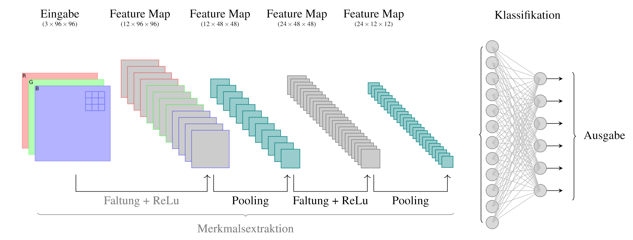
Beispielarchitektur

In der folgenden Beispielarchitektur wird ein RGB-Bild mit und einer von sechs Klassen zugeordnet.

Die Architektur könnte wie folgt aufgebaut sein:

• -Input
• Block 1
  • 12 Conv-Filter mit Kernel, padding=same und stride=1
  • ReLU
  • -Max-Pooling mit padding=same und stride=2
• Block 2
  • -Conv mit padding=same und stride=1
  • ReLU
  • -Max-Pooling mit padding=same und stride=4
• FCN
  • Fully-Connected-Layer mit 12 Neuronen
  • Softmax